After processing the document using computer vision, we have a list of tokens in the PDF. These tokens represent discrete bits of text within the document flow and generally correspond per word. For each, the robots have constructed a bounding polygon indicating where the word was detected on the page.

Natural language

A typical immunization record contains 500 to 1000 words. Most of these don't directly prove the student’s compliance calculation. We also capture letterhead, instructions, and other boilerplate and metadata.

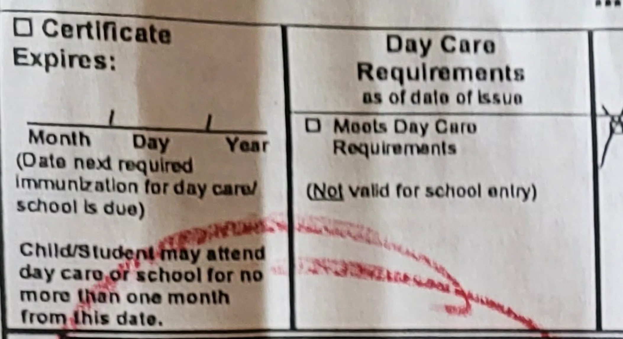
Our system doesn't consider metadata on the page like attested compliance status when parsing the document. We do infer expiration dates for all student documents, but there's a lot of room for interesting work in this area.

We can leverage this content to sharpen our machine intelligence in the future. For now, though, these unrelated tokens are just extraneous clutter. We thus must filter down the list to only those words or tokens that could affect immunization compliance.

In particular, we need to identify the subset of tokens describing:

1. the types of immunizations administered to the student or the shot types;

2. the dates that each immunization was administered or the shot dates;

3. and the student who owns the document or the subject

In each case, we use a different strategy to find the shot type, date, or student referenced in a text. We’ll discuss the specifics of matching each data type in future entries.

We use fuzzy logic to loosen the requirements to calculate a match to make our system more reliable. If we correct for typos and other lexical variations, we’re casting a wider net than with a less flexible approach. We inevitably produce more false positives by minimizing the number of false negatives.

Sorting true matches from false is critical. We deploy an iterative variation of the classic Karp-Rabin algorithm to do so efficiently.

A green approach

Let’s start simple. We need to identify the student who owns a given document.

First, we could compile a list of all the students' names in the school population. Then, we can examine each two-word subsequence within the flow of tokens in the document. When we find an exact match for the text in our list of names, we’ve found our student.

Bad news

This approach, while straightforward, performs poorly in practice. For a big district, a list with the names of every student would grow quickly and take up a lot of space on the computer. Comparing each token subsequence against each of these names or patterns would likewise take a long time.

If we look ahead to shot dates, the situation is grave for even the smallest schools. We expect every shot to happen within an 18-year historical window for current students. That span includes 6574 distinct dates. Each of the written date formats we support would need an entry or pattern in our list.

If a typical document contains 500 words, we can take the product of these lengths to show that we’d need to make about 3.25 million text comparisons to identify all dates within.

This program will take a long time. Fortunately, computer science exists mainly to make things faster. First, we must figure out exactly how bad things are now.

Big O-no!

Computer scientists characterize the performance of programs using Big-O notation. This is a special kind of mathematical function that describes a program's space or time complexity.

As the inputs to the program grow in size — the number of words or students in our case — this figure tells us how much time the program takes to finish or how much space the computer would use during. Because every computer offers different resources, we can’t give an exact number here. Instead, Big-O notation operates asymptotically and offers insight into program performance as input conditions approach infinity.

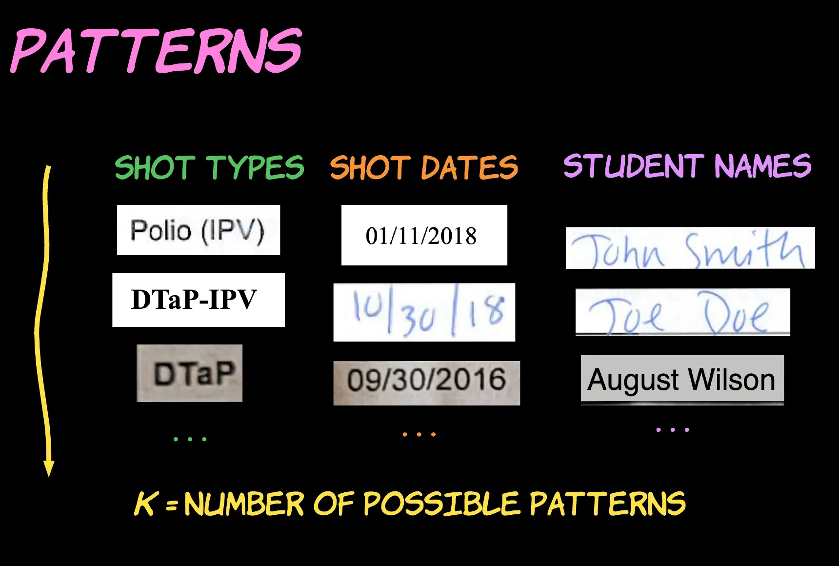
We define K to be the number of possible distinct patterns. This is the count of different shot types, the number of dates in the examined period, or the number of students who could be listed in the document.

Let’s say we have K entries in our list for comparison, each with J characters, and our document contains M words. We can express the relationship between the size of these inputs and the resulting time needed to run our program using Big-O notation.

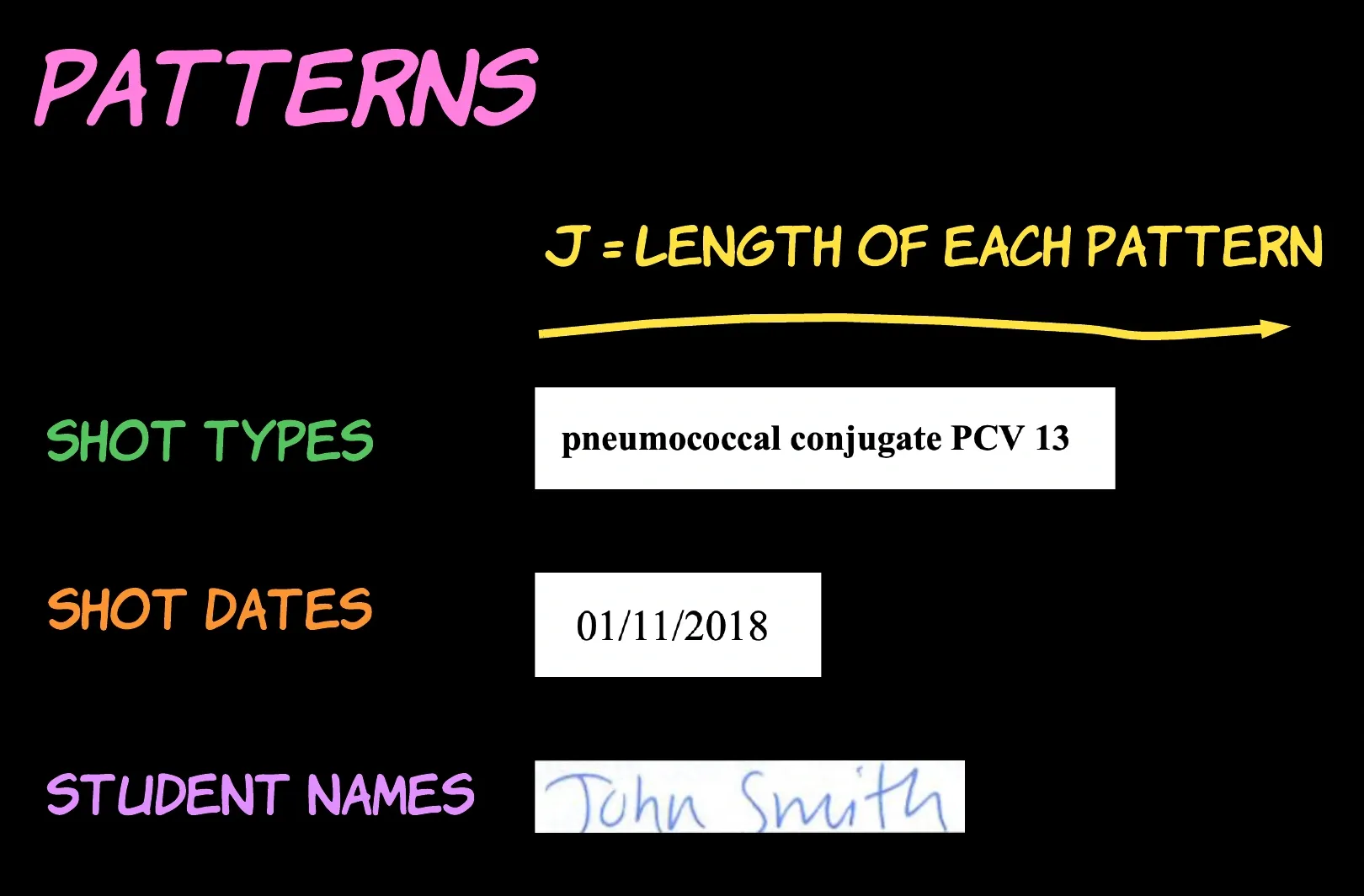
We define J to be the length of the possible patterns. This is the number of letters in the label of the shot type, the written date, or the student's name.

For a single pattern, we scan the M characters in the document and compare the length-J substring anchored at each position with our pattern, taking O(M + J) time. Repeating this process for each of the K patterns yields a total running time of O((M + J)*K).

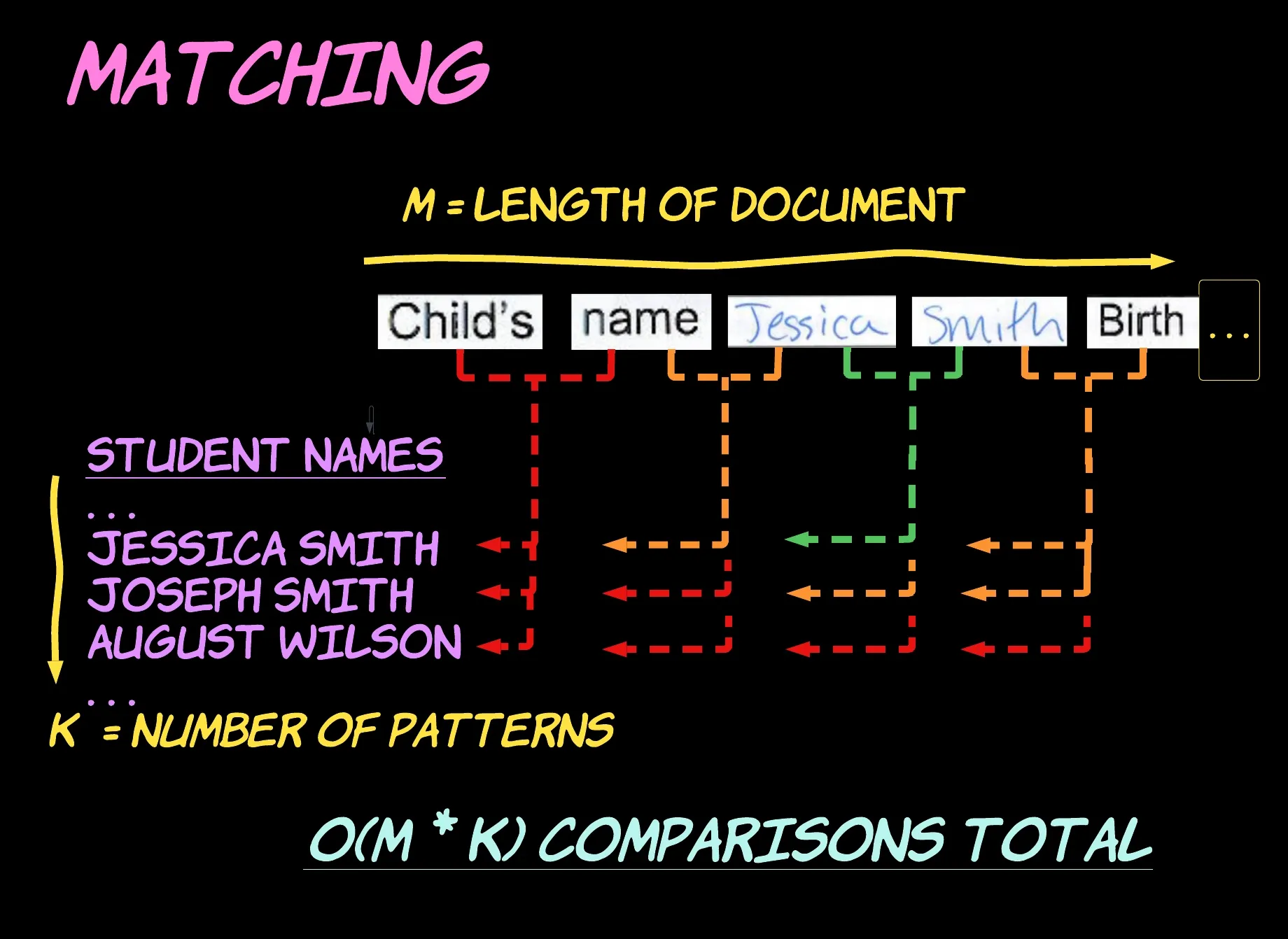
When scanning the document using our naïve strategy, we will perform a number of comparisons roughly equivalent to the length of the document multiplied by the number of patterns under inspection.

Getting better

The first step in performance optimization is determining the places in our program to prioritize for reformulation. Returning to our Big-O notation, we can see how each factor contributes to overall performance.

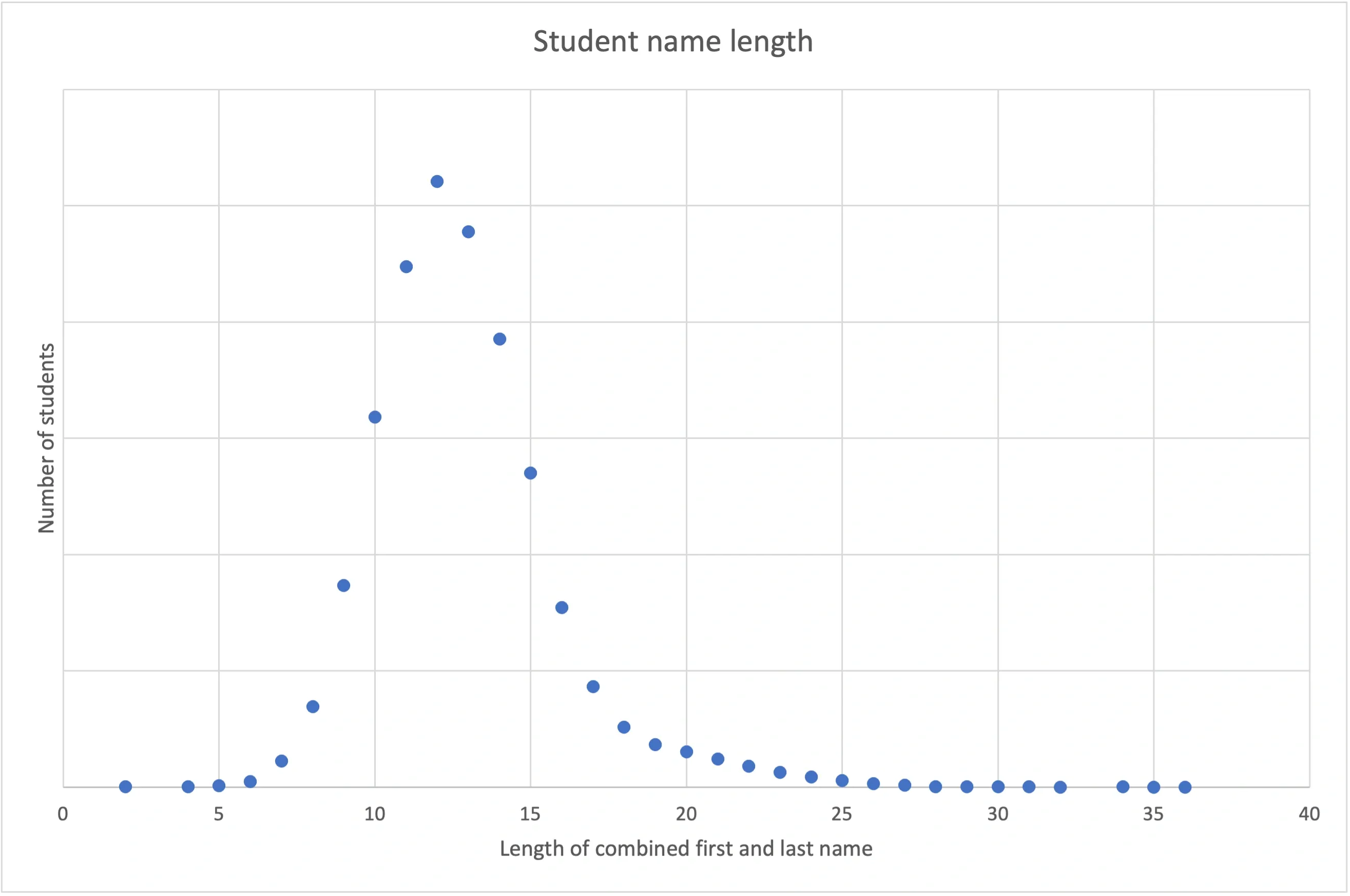
The chart above shows the distribution of the length of combined first and last names across a sample of students. It's unlikely we'll need to match a student whose name is longer than 35 characters.

For dates, names, and shot types, we expect the length of our patterns to match will remain fairly short. Optimizing the performance of our program for an increasing J won’t have much impact in practice on the program's complexity.

We could optimize two other factors: K, or the number of patterns for the comparison, or M, the length of the document.

Although our documents may contain many words, in practice, there’s a limit on the length of documents we observe in the wild. There is also a bound on the number of students we could need to compare, but it’s growing far faster over time as we serve bigger and bigger districts.

Taking this all together, it makes the most sense to optimize for K, the number of patterns for comparison.

Mo’ algos, mo’ problems

Generations of computer scientists have dedicated PhDs to finding faster ways to search for strings of characters within a larger body of text.

Somebody has to do it. Be grateful it isn't you.

In the case of matching on a single pattern — like the name of one student in particular — many algorithms use arcane math and implementations to improve performance over longer and longer texts. But we’re not searching for a single pattern; we have many!

In our situation, an “old” classic instead delivers superior results.

A load of Karp-Rabin

The Karp-Rabin algorithm was created in 1987 by Richard Karp and Michael Rabin, two computer scientists, and winners of the Turing Award. The algorithm is well-known for its spare and elegant approach and is taught widely in courses on algorithm design.

The algorithm relies on a rolling hash function to greatly reduce the number of comparisons the program needs to perform. Generally speaking, a hash function returns the same numeric hash value given the same argument. For two identical sequences of characters, a hash function will thus return the same number. We will apply our hash function to a moving window or subsequence within the input text. Rather than hashing the entire document into one value, we hash the text word-by-word, chunk-by-chunk.

We expect our pattern to comprise multiple words for names and shot types. If our window moves word-by-word, two patterns may have the same hash value over some subparts. For example, DTaP-HepB-IPV and DTaP-HepB-HepA could return the same hash value depending on the width of our window. Our hash function could return the same value over the segment “DTaP-HepB” regardless of anything written after.

This means our hash function may only indicate an approximate match. This is enough, however, to skip over most of the irrelevant content in the document. Instead of performing an expensive, exact comparison at every position in the text, we apply our hash function to successive chunks. If the hash function returns a value we recognize from our dictionary of patterns, we stop and perform a more exhaustive comparison.

Through this process, we can identify the boundaries between instances of patterns close together on the page. Using a similar “metal detecting” process to our initial tokenization, we determine the longest subsequences with the strongest matches.

Returning to our example, instead of calling the match “DTaP-HepB-IPV” when we see “DTaP,” our algorithm proceeds to consider “DTaP-HepB.” This may not be an exact match to any shot type. Even though the previous subsequence “DTaP” is an exact match, our algorithm continues to find the final element of the triplet “IPV.”

Because we design our system to prioritize longer pattern matches, we detect the shot-type “DTaP-HepB-IPV” rather than “DTaP,” “HepB,” and “IPV” separately. In the same way, we can correctly parse even an ambiguous string like “1 2 95 23 09 05” into a sequence of dates 1/2/1995 and 9/23/05

How did we do?

How we perform the exact match will vary between data. But generally, we can expect “metal detection” to take O(J*K) time at worst to compare each of the J length subsequences against our k patterns. We’ll repeat this process at each position in the length M document.

In the worst case, the document is full of names, dates, or shot types, all close together on the page. Then we could have to perform this exhaustive, expensive check at every position. This would imply a sluggish runtime of O(M*J*K). This is even worse than our original O((M+J)*K)!

Thankfully, this worst case is rare enough that it makes more sense to explore the expected or average performance under typical conditions instead. The number of dates, shot types, or names we expect to find in the document is constant to the length of the document. That is, more words on the page don’t strictly imply the student had more immunizations.

This means we’ll only need to perform the exhaustive comparison a handful of times throughout the document. We expect to attempt a quick approximate match at each of the M positions in the document, performing our O(J*K) exhaustive match only a constant number of times. This implies a total running time of O(J*K + M).

How does our new time O(J*K + M) compare to the original O(J*K + M*K)? The only difference is the second term, now M instead of M*K. Recalling the numbers for dates, a typical document contains 500 words (M) with 6574 possible shot dates (K). Because we’ve minimized the impact of the fastest-growing factor, K, we’ve reduced 3.25 million comparisons (M*K) to just 500 (M)

Not bad for a bit of fishing!

What's next

Karp-Rabin isn't very useful on its own. We need hash functions matching text with students, dates, and shot types. We'll start with shot types.